IDL最优估计(OE)函数中的几个例子

1 LMFIT函数
LMFIT函数对具有任意数量参数的函数进行非线性最小二乘拟合。LMFIT使用Levenberg-Marquardt算法，该算法结合了最速下降法和反黑塞斯函数拟合方法。该函数可以是任何非线性函数。算法执行迭代，直到三个连续的迭代未能将卡方值变化低于指定的阈值为止，或者直到执行了最大数量的迭代为止。
例子：
使用LM算法拟合公式：f(x)=a[0] * exp(a[1]*x) + a[2] + a[3] * sin(x)
偏导数计算公式：
dF(x)/dA(0) = exp(A(1)*X)
dF(x)/dA(1) = A(0)*X*exp(A(1)*X) = bx * X
dF(x)/dA(2) = 1.0
dF(x)/dA(3) = sin(x)

FUNCTION myfunct, X, A
; First, define a return function for LMFIT:
  bx = A[0]*EXP(A[1]*X)
   RETURN,[ [bx+A[2]+A[3]*SIN(X)], [EXP(A[1]*X)], [bx*X], $
      [1.0] ,[SIN(X)] ]
END
PRO lmfit_example
; Compute the fit to the function we have just defined. First,
; define the independent and dependent variables:
X = FINDGEN(40)/20.0
Y = 8.8 * EXP(-9.9 * X) + 11.11 + 4.9 * SIN(X)
measure_errors = 0.05 * Y
; Provide an initial guess for the function's parameters:
A = [10.0, -0.1, 2.0, 4.0]
fita = [1,1,1,1]
; Plot the initial data, with error bars:
PLOTERR, X, Y, measure_errors
coefs = LMFIT(X, Y, A, MEASURE_ERRORS=measure_errors, /DOUBLE, $
   FITA = fita, FUNCTION_NAME = 'myfunct')
; Overplot the fitted data:
OPLOT, X, coefs
END

2 CURVEFIT函数
CURVEFIT函数使用梯度扩展算法来计算与具有任意数量参数的用户提供的函数的非线性最小二乘拟合。用户提供的函数可以是偏导数已知或可以近似的任何非线性函数。执行迭代，直到卡方小于指定的阈值，或者直到执行了最大数量的迭代为止。
例子1：
拟合公式：F(x) = a * exp(b*x) + c
偏导数计算：
df/da = EXP(b*x)
df/db = a * x * EXP(b*x)
df/dc = 1.0

PRO gfunct, X, A, F, pder
  bx = EXP(A[1] * X)
  F = A[0] * bx + A[2]
;If the procedure is called with four parameters, calculate the
;partial derivatives.
  IF N_PARAMS() GE 4 THEN $
    pder = [[bx], [A[0] * X * bx], [replicate(1.0, N_ELEMENTS(X))]]
END
Pro CURVEFIT
X = FLOAT(INDGEN(10))
Y = [12.0, 11.0, 10.2, 9.4, 8.7, 8.1, 7.5, 6.9, 6.5, 6.1]
;Define a vector of weights.
weights = 1.0/Y
;Provide an initial guess of the function’s parameters.
A = [10.0,-0.1,2.0]
 
;Compute the parameters.
yfit = CURVEFIT(X, Y, weights, A, SIGMA, FUNCTION_NAME='gfunct')
 
;Print the parameters returned in A.
PRINT, 'Function parameters: ', A
End

输出结果：
Function parameters: 9.91120 -0.100883 2.07773
最终拟合结果：
f (x) = 9.91120(e-0.100883x) + 2.07773
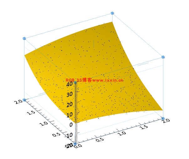
例子2：
拟合公式Z = A X^B + C X Y + D Y^E

PRO mymulticurvefit, XY, A, F, PDER
     X = XY[*,0]
     Y = XY[*,1]
     F = A[0]*X^A[1] + A[2]*X*Y + A[3]*Y^A[4]
     PDER = [[X^A[1]], [A[0]*X^A[1]*ALOG(X)], $
     [X*Y], [Y^A[4]], [A[3]*Y^A[4]*ALOG(Y)]] 
END
Pro CurvefitTest2
seed = 1
n = 1000
X = 2*RANDOMU(seed, n)
Y = 2*RANDOMU(seed, n)
XY = [[X], [Y]]
A = [-3, 2, 5, 3, 3]
noise = RANDOMN(seed, n)
Z = A[0]*X^A[1] + A[2]*X*Y + A[3]*Y^A[4] + noise
;Provide an initial guess of the function's parameters. 
A = [1d, 1, 1, 1, 1]
;Compute the parameters. 
yfit = CURVEFIT(XY, Z, weights, A, $
FUNCTION_NAME='mymulticurvefit') 
PRINT, 'Function parameters: ', A 
; Plot the original data as scattered points.
iPlot, X, Y, Z, /SCATTER
; Create a 2D surface of the final fit.
X1 = 2*FINDGEN(101)/100
X = REBIN(X1, 101, 101)
Y = TRANSPOSE(X)
Z = A[0]*X^A[1] + A[2]*X*Y + A[3]*Y^A[4] 
iSurface, Z, X1, X1, /OVERPLOT
END

喜欢 (1)赏

支付宝[853060844@qq.com]

分享 (0)